
Are you stuck with the concept of Excel VLookUp Function? Then here is your Ultimate Guide to use Excel VLookUp Function like a Pro.
Most of the learners have been complaining about understanding the real working of Excel VLookUp Function. If a user wants to retrieve the value from a cell and then wants to use the same value in somewhere else in the Excel sheet, Excel VLookUp Function can be useful in such cases. When it comes to data analysis, professional always go for Excel VLookUp Function.
Most beginners think that this function is some kind of complicated science, but in reality, it is going to be fun learning the working of Excel VLookUp Function. Let’s get started with a detailed overview of this function:
Excel VLookUp Function
To understand the simplistic function of Excel, the VLookUp Function considers it like a search tool that looks for a specific value in the given data in the Excel sheet. Once it finds the required value, it extracts the useful information too that is associated with that value.
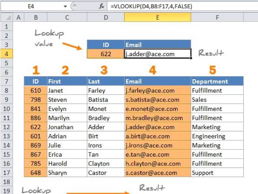
Real World Example
Imagine you have two separate spreadsheets, one with the clients’ data and the second one with the revenue data. With the help of this formula, you can extract the revenues from that spreadsheet and compare with the client data. In this way, you get a more significant and clear understanding of the data.
Working with Excel VLookUp
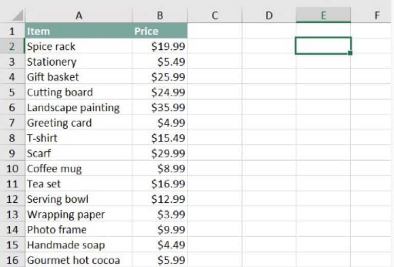
We will try to understand the working of this formula with the help of an example so you can get a better and clear concept of this function. If you run a shop and have added the items on a list with the price tags, you can use this VLookUp formula to know the price of any specific item on that list.
In the example given below, imagine that we are asked to find the value of the photo frame. If there is a large amount of data, then it is going to be impossible to scroll through the sheet to find that value. That’s why Excel VLookUp Function is used to get rid of complex processes and time taking procedures. Once you have understood the formula, it will be straightforward for you.
Here, we are going to use the formula in E2 cell, but you can use it in an empty cell. This formula will also start with a traditional equal sign (=). After that, type in the name of our formula. Now, the arguments are going to be written in parenthesis so write the open parenthesis (or bracket). At this step, our formula will be like this
=VLOOKUP(
Adding Arguments
Now let’s go for adding the arguments. These added arguments will guide the VLookUp function that what we are going to search for and what we are searching. The name of your item is going to be the first argument here. As the name of the item is photo frame so it will look like this:
=VLOOKUP(“Photo frame”
Now, it turns for the second argument, and that is the cell range in which the data lies. The user must use a comma to separate each argument. As per our given data:
=VLOOKUP(“photo frame”, A2:B16
The column index number is the third argument in the VLookUp Excel function. It is pretty simple as the 1st column in the given range is 1, and the 2nd column is 2. So, our thirds argument will be 2 as the second column contains the prices of the items.
=VLOOKUP(“photo frame”, A2:B16, 2
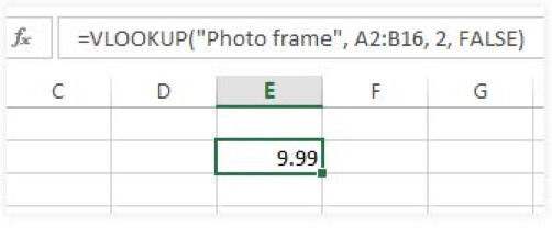
The approximate match is determined with the help of the fourth argument. It can be false or true. If the argument is true, then it will go for approximate matches. As our requirement is exact math, so this argument is going to be False. Now close the parenthesis, and the exact Excel VLookUp function would look like this:
=VLOOKUP(“photo frame”, A2:B16, 2, FALSE)
When the user presses the enter key, a similar result will be shown to the user.
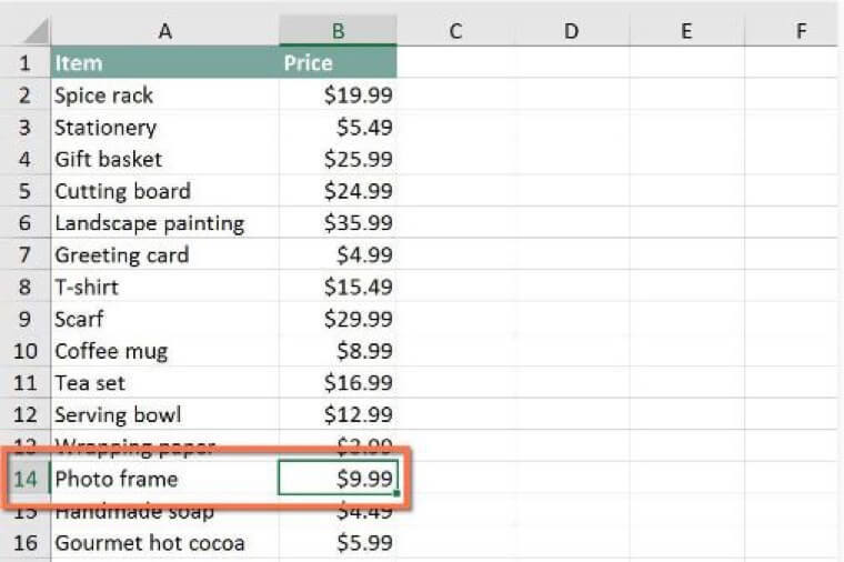
How VLookUp Works?
The VLookUp formula will search vertically for the desired item in the first column. As soon as it finds the word, photo frame, it will move forward to the 2nd column to show the price.
If you want to go for any other item, it will be easier for you as you just need to replace the name with that exact keyword. Just imagine that you want to use Excel VLookUp function to find the value of T-Shirt from the given data. Now, remove the photo frame from the given formula and replace it with T-shirt.
Now for the T-shirt, the Excel VLookUp function would look like this:
=VLOOKUP(“T-shirt”, A2:B16, 2, FALSE)
Use of VLookUp Function
Instead of doing everything manually, Excel VLookUp Function makes things easier and faster. If you want to find a specific value from a given data or hundreds of columns, VLookUp Function will reduce the task to few clicks only. In the beginning, it may seem like a hard task after enough practice, you will master the art of Excel VLookUp Function, and you will find it very useful.
We hope that this guide has been beneficial as every single step and working is described in details. There is a lot to learn about VLookUp Function yet, and you can unleash the real power of VLookUp Function in different situations and become an Excel Expert.
Want to learn more about what the differences are between VLookUp and Index Match functions? Then don’t miss this post.